Augmented Search capacity planning
Deploying a powerful search offers an opportunity to greatly improve the end-user experience but can also introduce new challenges primarily associated with performance of the search backend.
Due to the nature of the operations being performed and the high performance of its querying system, Elasticsearch capacity planning can be complex as you try to achieve the right balance between the size of the dataset and cluster size.
This topic discusses factors to consider when sizing your environment (Elasticsearch primarily) for Augmented Search as well as design considerations potentially impacting performance.
Indexing vs. querying
As with any data store, there are two types of operations performed by Augmented Search:
- Indexing
includes operations associated with extracting data from a Jahia page to make it searchable. - Querying
includes operations associated with fetching data either in the form of search results or aggregations (for example, the number of documents created by all authors on the platform).
In Augmented Search, indexing can be performed either in bulk (for example when a new site is imported), or on-the-fly as documents are saved (and/or published) by the content editor.
While querying and single document indexing must be sub-second operations (and generally sub-200ms operations), bulk indexing operations can sometimes take hours depending on the size of the dataset to index.
Indexing considerations
As the volume of data to index has a direct impact on bulk indexing time, ensure that only the content that needs to be searchable is sent for indexation. Keep in mind that what might not be critical for single document indexing can easily become a challenge when this operation has to be repeated a million times.
When configuring Augmented Search, be conservative by only using data actually required to build your search experience and avoid indexing data you might need later.
The following settings in the Augmented Search configuration file (org.jahia.modules.augmentedsearch.cfg) have a direct impact on the amount of data that is indexed.
| Property | Description |
|---|---|
| indexParentCategories | Indexes all ancestors as well as the category itself |
| content.mappedNodeTypes | Indexes additional properties to make them available for faceting or filtering. |
| content.indexedSubNodeTypes | Aggregates subnodes properties alongside their main resource in the indexed document |
| content.indexedMainResourceTypes | Nodes to be indexed as main resource |
| content.indexedFileExtensions | File extensions to be indexed |
| workspaces | Specifies the workspace to be indexed (ALL or LIVE only) |
Indexing features
To provide more granularity for its indexing operation, Augmented Search offers the ability to trigger indexing by site and workspace.
Indexing per site
Using our configuration UI (Jahia 8.X only) with site-admin pemission or using our GraphQL API (Jahia 7.X or Jahia 8.X), you can trigger indexing for one site, multiple sites, or all sites at once. This example shows how to index only the digitall site.
mutation { admin { search { startIndex(siteKeys: ["digitall"]) } } }
Note that Augmented Search indexes sites serially (one site at a time). Therefore, the time it takes to index all your sites in bulk is identical to the sum of indexing all sites individually. The flexibility lies in the ability to reindex only a portion of the dataset to limit the impact indexing operations have on the infrastructure.
Indexing per workspace
You can also trigger bulk indexing only for a particular workspace. This example shows how to index the live workspace for the digitall site.
mutation { admin { search { startIndex(siteKeys: [“digitall”], workspace: LIVE) } } }
Cluster sizing
With Augmented Search, you can run bulk indexing operations without impacting querying capabilities. Bulk indexing performs the indexing operation and creates a new index. Once indexing is successful, Augmented Search redirects queries to the new index and deletes the old one. This means that your cluster must be able to hold at least twice the amount of data during the indexing operation.
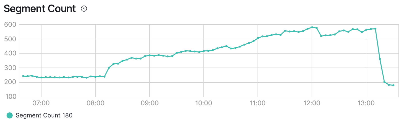
A reindexing operation across all sites
Querying consideration
Query-time performance, key to a positive user experience when searching, is typically measured in the number of milliseconds it takes for the response to come back after user interaction (usually a user typing a search query).
In most cases, connectivity and operations performed by resources on the path between a user and the data store are not the source of increased latency (other than a few milliseconds). With Jahia, data transits between the user and a Jahia server (eventually through a reverse proxy). Jahia analyzes the GraphQL query, converts it into an Elasticsearch query, sends it to Elasticsearch for processing, and then sends it all the way back again.
The complexity of an operation also has an impact on performance. The more complex an operation is, the longer it takes for Elasticsearch to process it and return a response. For example, if performing an aggregation on a field takes 150ms, performing the same aggregation on two different fields is likely going to take 300ms, and so on. Also, when complex queries run, the load on Elasticsearch increases accordingly, reducing the available compute time for other users.
In short, if your server can process 10 units of processing per second and a query consumes 1 unit, you can serve 10 users in that interval. But, if a query consumes 4 units, you will only be able to serve 3 users in that same interval.
Finally, the size of the dataset compared to the actual technical specifications (CPU, RAM, and disk of the Elasticsearch cluster nodes) also plays an important role in the capacity of the server to process queries efficiently.
To sum, the following factors are important (in no particular order):
- Processing cost of the query
- Size of the dataset
- Load on the server
- Cluster technical specifications
Elasticsearch sizing
The good news is that Elasticsearch scales very well horizontally. Adding more resources (more nodes) to an Elasticsearch cluster is generally an answer to performance or load issues.
With Jahia, the operations performed during search are not compute intensive and we didn’t run in a situation where Jahia represented a significant bottleneck. However, adding more resources can also quickly become very costly, thus the need to optimize querying.
Query and UI optimization
When designing a search experience, developers should consider resource utilization and optimize querying to avoid unnecessary loads on the infrastructure, or even better, optimize querying to avoid performing operations that fetch data users are unlikely to need. This is not just a developer’s concern. UI/UX designers should also consider the impact their design has on the infrastructure.
Search-as-you-type, the Google example
Search-as-you-type is a good example of a search experience that can potentially become very expensive if not implemented properly.
For example, Google built their search experience to optimize consumption on their infrastructure (of course!) while providing a good user experience. As you start typing a query, Google gives you clues about search terms associated with what you typed, but does not actually give you more than the title, and eventually a subtitle and an image. As a user types search criteria, many micro-requests are generated for the Google infrastructure. By reducing the query scope, Google also reduces loads on the server.
If we push the logic even further, it’s also more than likely that by recommending results during initial search, Google actually aims at redirecting users to cached content. This makes it less expensive when a user clicks on a recommended search term, rather than processing every custom search term entered by the visitor.
Then, and only then, when you click Enter (or the magnifying glass), does Google perform a query fetching a lot more information about the search terms (including a title, thumbnails, search excerpt, and other metadata). This expensive operation is kept until the very last moment, hoping that the search term actually corresponds to what the user is looking for, and limiting the need to further refine (and perform additional expensive queries).
Here are some factors to consider when building your search experience:
- Use different queries (and different results) for search-as-you-type than your full search page (containing facets, filters, and more)
- Don’t fetch facets by default. Let the user enter search terms first, then perform aggregation on the content.
- Tweak the delay between keystrokes before actually triggering a search. If a user is interested in tomatoes, wait for them to enter the full word instead of triggering a search on each keystroke (“t”, “to”, “tom”). You can also wait for a particular delay after the last keystroke.
This doesn’t mean you absolutely have to follow these recommendations. If search is a key element of your platform and your infrastructure is sized accordingly, you could offer a very detailed search experience from the start.
No one-fit-all solution
As you might guess from the various factors covered previously, sizing an Elasticsearch cluster is a complex exercise and depends on a wide variety of factors unique to each environment. The structure of your data, the amount of it, and the queries you are going to perform, all play an important role in determining the ideal cluster size.
Before jumping into Augmented Search, we understand that it is essential to understand its resource needs. Instead of providing generic numbers that might be approximate, we’ve decided to provide benchmark results with a variety of scenarios to allow you to relate your implementation needs to the dataset we tested and to understand associated boundaries.
Benchmarking
Approach
Our primary objective when creating our test runs (using JMeter) is to progressively increase the query load until the Elasticsearch cluster reaches 100% CPU utilization, and collect mean response times and error rates associated with a particular throughput during that time.
Using a ramp-up time of 90 seconds, we progressively increased the sample size (count of API calls) and monitored the behavior on a wide variety of queries.
| Sample size | Error count | Latency | Throughput |
|---|---|---|---|
| 1000 | 0 | 277 | 11 |
| 2000 | 0 | 278 | 22 |
| 3000 | 0 | 300 | 33 |
| 4000 | 0 | 323 | 43 |
| 5000 | 0 | 2157 | 55 |
| 6000 | 0 | 21127 | 54 |
| 7000 | 1465 | 27645 | 70 |
Results of a term aggregation query
Generally, the latency increases progressively alongside the load until the system reaches a point (usually at 100% CPU consumption) at which it cannot process the requests fast enough. Then, the system starts piling them up (which results in increased latency) until it cannot handle it anymore and starts erroring out.
The above results are a typical illustration, the latency increases slightly until reaching a sample size of 4000 API calls (with a mean latency of 323ms at 43 queries per second). The next two samples (5000 and 6000) do not error out, but latency is through the roof (and is not usable in production). Also notice that these two runs have an almost identical throughput, which corresponds to the system’s max capacity.
Finally at 7000, the API starts crashing, with 1,465 failed calls out of the 7000. Interestingly, at sample size the throughput is increasing, but that is simply because the server is refusing calls “Nope, too busy! Come back later”.
When analyzing test results, we’re looking for the time when multiple runs are getting a similar throughput, which usually corresponds to the throughput of the system when operating at its maximum capacity.
For the results above, the number we’ll keep for our metrics is 55 queries per second.
Queries and search terms
To provide accurate results, we ensured that search terms match actual content (queries with 0 results use less resources). In the context of these benchmarks, we ran all queries in 4 different languages (German, English, French, and Portuguese) using 6 different search strings per language. When performing aggregations or filters, we ensured these were also matching content on the sites.
As for the queries, we performed the runs with 7 different queries with different levels of complexity:
| Query Name | Description |
|---|---|
| Simple search | Performs a simple search in a set language and returns a name, excerpt, and path. This is the most common search experience. |
| Two filters | Adds two filters (on author and publication date range) to “Simple search”. Returns the pages created by John D. between November 15, 2020 and February 15, 2021 matching a set query string. |
| Range facet | Performs a range aggregation (over 8 buckets) in addition to “Simple search” |
| Term facet | Performs a term aggregation, by author, in addition to “Simple search” |
| Tree facet | Performs a tree aggregation by categories (similar to term facet but identify if the tree element has any children), in addition to “Simple search” |
| Range facet with two filters | Performs a “Simple Search”, “Range facet” and “Two filters” in the same query |
| Three facets | Performs a “Simple Search” Range facet”, “Term facet” and “Tree facet” in the same query. |
During our benchmarks, we also performed a run while indexing was occurring to measure the impact of whole-site indexing on search queries.
Data caveats
These tests represent a snapshot of an environment at a particular point in time with a particular dataset and are not going to be perfectly reproducible (even with the same environment). You will get different results!
In these benchmarks, the throughput is expressed in queries/second, and should not be confused with the ability of the Jahia platform to serve a specific number of users per second. This throughput corresponds to the number of API calls processed by Augmented Search (for example, users all clicking on the search button at the same second).
Remember that these numbers correspond to the maximum throughput and should not be used to define a nominal production environment. We recommend lowering these numbers by 25-30% for nominal production to keep room for an unplanned increase of traffic.
Testing infrastructure
The following environment was used for the tests:
- Elasticsearch cluster: 3x 8GB RAM, 240GB SSD using AWS “aws.data.highio.i3” instance
- Jahia cluster: 2x 8 Cores 8GB RAM, SSD storage (1 browsing/authoring + 1 processing)
- Jahia database: 3x 8 Cores 8GB RAM, SSD storage
- Jmeter host: 1x 32 Cores, 64 GB RAM using AWS “c5a.8xlarge”
Understanding the data
Consider the following factors when reviewing the runs results:
- Search Hits
Number of elements searchable through Augmented Search API across the entire platform. One page translated in 15 different languages and available in both live and edit workspaces will account for 30 search hits. - Mean
Mean response time in milliseconds across all queries for the particular batch. For example, if performing a batch of 5000 API calls within 90 seconds, mean corresponds to the mean over the 5000 queries. - 95th %ile
Mean response time in milliseconds across the 95% of the slowest responses for the batch. - Recommended
The recommended value corresponds to results with the 95th percentile below 500ms - Max
Without considering latency, the maximum throughput obtained without API errors. This gives a notion of the potential maximum that the system can support.
Since we execute our tests in batch of API calls (for example 1000, 2000, and 3000) with a fixed ramp-up time (90s), we get a good understanding of the maximum throughput supported by the system, but we can’t get precise latency measurements for every single increment in measured throughput.
For illustrative purposes, we performed a run with 200 calls increments, which provides a good sample of results across all runs. Below, note the recommended and max values. Notice that soon after the max, the 95th percentile latency increases significantly, and then starts erroring out around the 6600 sample count.
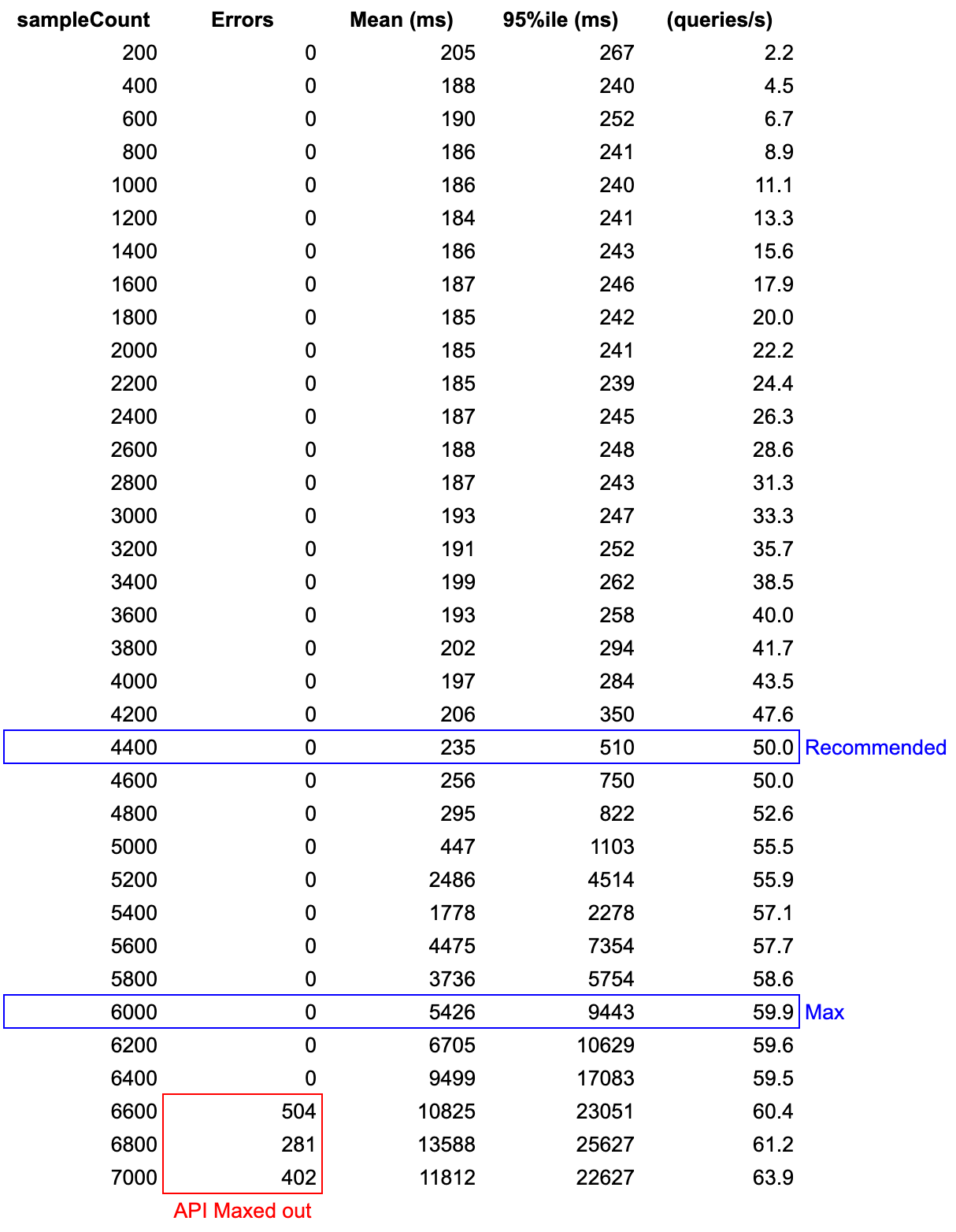
Run results
Remember, we are submitting the sample count within a 90 seconds window. Compare the measured throughput versus the average rate of submitted calls (sampleCount/90s) and notice that the two lines diverge at 5000 samples. At this time, the API is unable to process the data in “real-time” and begins queuing API calls.
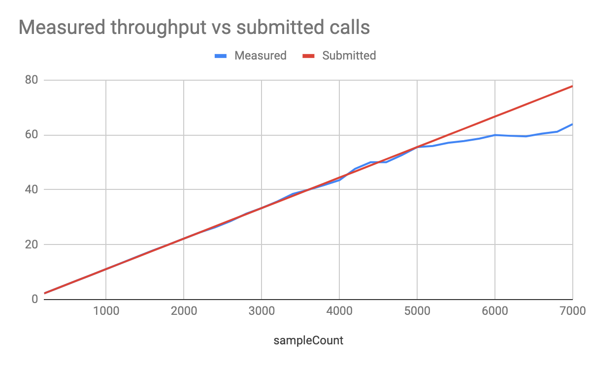
Also notice that our recommendation is for 50 q/s (4400 samples) while the real-time max is actually at 55.5 (5000 samples). The reason here is that we want as much as possible to avoid going much over 500ms latency.
Run #1
| Number of ES Documents | Dataset size | Search Hits |
|---|---|---|
| 7,890,693 | 9.9 GB | 239,043 |
| Number of ES Documents | Nominal | During query benchmark |
|---|---|---|
| Indexing time | 1 hour 10m | 1 hours 18m |
| Query | Throughput (queries/second) | |||
|---|---|---|---|---|
| Nominal | During indexation | |||
| Recommended | Max | Recommended | Max | |
| Simple Search | 67 q/s 95th %ile: 594ms Mean: 195ms |
90 q/s 95th %ile: 5214ms Mean: 3795ms |
63 q/s 95th %ile: 358ms Mean: 174ms |
67 q/s 95th %ile: 1024ms Mean: 246ms |
| Two filters | 56 q/s 95th %ile: 202ms Mean: 156ms |
89 q/s 95th %ile: 4634ms Mean: 3209ms |
63 q/s 95th %ile: 318ms Mean: 176ms |
77 q/s 95th %ile: 1264ms Mean: 264ms |
| Range facet | 43 q/s 95th %ile: 594ms Mean: 269ms |
50 q/s 95th %ile: 10637ms Mean: 6915ms |
33 q/s 95th %ile: 354ms Mean: 253ms |
36 q/s 95th %ile: 19876ms Mean: 12026ms |
| Term facet | 43 q/s 95th %ile: 323ms Mean: 238ms |
55 q/s 95th %ile: 2157ms Mean: 1048ms |
28 q/s 95th %ile: 508ms Mean: 272ms |
36 q/s 95th %ile: 21027ms Mean: 14403ms |
| Tree facet | 43 q/s 95th %ile: 427ms Mean: 253ms |
55 q/s 95th %ile: 2326ms Mean: 964ms |
28 q/s 96th %ile: 771ms Mean: 305ms |
51q/s 95th %ile: 9362ms Mean: 6253ms |
| Range facet with two filters | 43 q/s 95th %ile: 314ms Mean: 232ms |
56 q/s 95th %ile: 926ms Mean: 337ms |
33 q/s 95th %ile: 316ms Mean: 236ms |
47 q/s 95th %ile: 16386ms Mean: 8811ms |
| Three facets | 22 q/s 95th %ile: 755ms Mean: 438ms |
24 q/s 95th %ile: 18954ms Mean: 12531ms |
11 q/s 95th %ile: 859ms Mean: 495ms |
17 q/s 95th %ile: 31109ms Mean: 19099ms |
| Run Analysis |
|---|
The following deductions can be made from this run:
|
Run #2
| Number of ES Documents | Dataset size | Search Hits |
|---|---|---|
| 14,585,551 | 19 GB | 549,171 |
| Number of ES Documents | Nominal | During query benchmark |
|---|---|---|
| Indexing time | 4 hours 53 mn | 5 hours 3 mn |
| Query | Throughput (queries/second) | |||
|---|---|---|---|---|
| Nominal | During indexation | |||
| Recommended | Max | Recommended | Max | |
| Simple search | 63 q/s 95th %ile: 488ms Mean: 184ms |
77 q/s 95th %ile: 2340ms Mean: 409ms |
63 q/s 95th %ile: 633ms Mean: 237ms |
67 q/s 95th %ile: 23547ms Mean: 11358ms |
| Two filters | 62 q/s 95th %ile: 482ms Mean: 186ms |
77 q/s 95th %ile: 780ms Mean: 210ms |
63 q/s 95th %ile: 458ms Mean: 192ms |
66 q/s 95th %ile: 929ms Mean: 359ms |
| Range facet | 43 q/s 95th %ile: 305ms Mean: 242ms |
55 q/s 95th %ile: 2924ms Mean: 2281ms |
28 q/s 95th %ile: 496ms Mean: 267ms |
40 q/s 95th %ile: 10324ms Mean: 7411ms |
| Term facet | 43 q/s 95th %ile: 395ms Mean: 252ms |
55 q/s 95th %ile: 12779ms Mean: 7920ms |
28 q/s 95th %ile: 305ms Mean: 233ms |
36 q/s 95th %ile: 19539ms Mean: 6386ms |
| Tree facet | 43 q/s 95th %ile: 519ms Mean: 267ms |
55 q/s 95th %ile: 13353ms Mean: 8393ms |
28 q/s 96th %ile: 362ms Mean: 247ms |
38q/s 95th %ile: 14958ms Mean: 11154ms |
| Range facet with two filters | 43 q/s 95th %ile: 285ms Mean: 225ms |
60 q/s 95th %ile: 3181ms Mean: 2554ms |
33 q/s 95th %ile: 296ms Mean: 236ms |
42 q/s 95th %ile: 4961ms Mean: 3215ms |
| Three facets | 22 q/s 95th %ile: 686ms Mean: 422ms |
26 q/s 95th %ile: 9610ms Mean: 6559ms |
11 q/s 95th %ile: 1051ms Mean: 529ms |
17 q/s 95th %ile: 26802ms Mean: 13018ms |
| Run Analysis |
|---|
| For this run deductions from run #1 are still mostly valid. Note that the query that seems to be most impacted by the increase in the dataset size is the simple search, while all the aggregations behave very similarly. When performing free text search, the system has to search through a wide variety of elements (which increased alongside the dataset), while the fields being aggregated on are not seeing much variation in their content. Since run #1 is a subset of the data in run #2, the number of unique values for the authors fields are similar. As the site is larger in run #2, there are more documents for each author but a similar number of authors. |
Run #3
| Number of ES Documents | Dataset size | Search Hits |
|---|---|---|
| 21,772,140 | 347.1 GB | 1,660,897 |
| Number of ES Documents | Nominal | During query benchmark |
|---|---|---|
| Indexing time | n/a | 17 hours 22mn |
| Query | Throughput (queries/second) | |||
|---|---|---|---|---|
| Nominal | During indexation | |||
| Recommended | Max | Recommended | Max | |
| Simple search | 43 q/s 95th %ile: 251ms Mean: 193ms |
62 q/s 95th %ile: 1641ms Mean: 664ms |
44 q/s 95th %ile: 328ms Mean: 192ms |
62 q/s 95th %ile: 2419ms Mean: 882ms |
| Two filters | 63 q/s 95th %ile: 402ms Mean: 189ms |
77 q/s 95th %ile: 1719ms Mean: 322ms |
56 q/s 95th %ile: 522ms Mean: 246ms |
63 q/s 95th %ile: 1114ms Mean: 350ms |
| Range facet | 22 q/s 95th %ile: 491ms Mean: 340ms |
29 q/s 95th %ile: 15288ms Mean: 9591ms |
28 q/s 95th %ile: 424ms Mean: 267ms |
Same as recommended, errors if above |
| Term facet | 22 q/s 95th %ile: 526ms Mean: 333ms |
31 q/s 95th %ile: 10326ms Mean: 6668ms |
28 q/s 95th %ile: 280ms Mean: 232ms |
32 q/s 95th %ile: 8056ms Mean: 6444ms |
| Tree facet | 22 q/s 95th %ile: 468ms Mean: 326ms |
32 q/s 95th %ile: 7388ms Mean: 4679ms |
28 q/s 96th %ile: 288ms Mean: 239ms |
33q/s 95th %ile: 1915ms Mean: 908ms |
| Range facet with two filters | 22 q/s 95th %ile: 491ms Mean: 340ms |
29 q/s 95th %ile: 15288ms Mean: 9591ms |
28 q/s 95th %ile: 504ms Mean: 282ms |
37 q/s 95th %ile: 14138ms Mean: 8394ms |
| Three facets | 11 q/s 95th %ile: 1124ms Mean: 686ms |
Same as recommended, errors if above | 11 q/s 95th %ile: 741ms Mean: 454ms |
25 q/s 95th %ile: 14294ms Mean: 8740ms |
| Run Analysis |
|---|
| This run stretches the system in terms of capacity. For such a project, we would recommend deploying additional Elasticsearch resources if building a search experience making use of aggregations. |
Run #4
This last run was performed with increased Elasticsearch resources to measure impact on performance (3x 15GB RAM, 480GB SSD using AWS “aws.data.highio.i3” instance).
| Number of ES Documents | Dataset size | Search Hits |
|---|---|---|
| 21,772,140 | 347.1 GB | 1,660,897 |
| Number of ES Documents | Nominal | During query benchmark |
|---|---|---|
| Indexing time | n/a | n/a |
| Query | Throughput (queries/second) | |||
|---|---|---|---|---|
| Nominal | During indexation | |||
| Recommended | Max | Recommended | Max | |
| Simple search | 63 q/s 95th %ile: 589ms Mean: 225ms |
91 q/s 95th %ile: 4277ms Mean: 1803ms |
n/a (not tested) | n/a (not tested) |
| Two filters | 63 q/s 95th %ile: 423ms Mean: 181ms |
90 q/s 95th %ile: 4034ms Mean: 2172ms |
n/a (not tested) | n/a (not tested) |
| Range facet | 42 q/s 95th %ile: 422ms Mean: 314ms |
50 q/s 95th %ile: 2549ms Mean: 938ms |
n/a (not tested) | n/a (not tested) |
| Term facet | 42 q/s 95th %ile: 490ms Mean: 307ms |
53 q/s 95th %ile: 1333ms Mean: 568ms |
n/a (not tested) | n/a (not tested) |
| Tree facet | 42 q/s 95th %ile: 538ms Mean: 329ms |
53 q/s 95th %ile: 1194ms Mean: 529ms |
n/a (not tested) | n/a (not tested) |
| Range facet with two filters | 56 q/s 95th %ile: 531ms Mean: 261ms |
76 q/s 95th %ile: 2068ms Mean: 1568ms |
n/a (not tested) | n/a (not tested) |
| Three facets | 11 q/s 95th %ile: 687ms Mean: 498ms |
24 q/s 95th %ile: 1378ms Mean: 737ms |
n/a (not tested) | n/a (not tested) |
| Run Analysis | ||||||||||||
|---|---|---|---|---|---|---|---|---|---|---|---|---|
|
Run #4 should be looked at in comparison to run #3 since the two are using the same dataset, the only difference being in more resources given to the Elasticsearch cluster. We can see an increase in throughput, which was expected, but what is interesting to pay attention to here is the ability of the system to cope under load, which is especially noticeable in the 95th %ile and Mean latency for the Max “column”. Example with range facet query
|
Test summary
The four runs that were executed during this series of benchmarks should provide you with a good baseline to understand the expected performance of your search environment.
Three different datasets were analyzed (239,043 hits, 549,171 hits and 1,660,897 hits) and by reviewing both your dataset size, your desired performance and the type of search queries being performed you will get a good sense of either the resources needed or the expected performance.